NSRWNavier–Stokes Research Workbench
Explore NSRW
EQUATION → PROOF → CODE → SCIENTIFIC USE

When mass cancels,
angular history
stays positive.

A mathematical finding. An executable research path.

Starting from OpenAI’s outgoing-profile construction, NSRW derived and formalized a separation between mass and angular histories—then strengthened it into a quantitative bound and rigorous numerical code.

Flamehaven · Research snapshot: 31 October 2026 · Software v0.5.0
01 / RESEARCH CONTEXT

Begin with the equations.
Make the mathematics executable.

Navier–Stokes connects the evolution of incompressible velocity to transport, pressure, viscosity and forcing. It is the scientific setting for NSRW’s longer research program.

∂tu+(u·∇)u=−∇p+νΔu+f∇·u=0

u: velocity · p: pressure · ν: kinematic viscosity · f: forcing

The present study isolates the moment structure of one pinned construction. A source Profile fixes tail and schedule data, a coefficient bound and a consistent angular-reset witness. Its repair pulses enforce terminal history constraints.

THE PROGRAM

Build results that can become useful operations.

NSRW asks mathematical questions, tests candidate assumptions, derives surviving consequences and turns them into checked proofs and evaluable code.

The destination is practical scientific computation: quantities, error bounds and diagnostics that another researcher or developer can call, inspect and compare in a real workflow.

Equation to Artifact roadmap ↗
02 / MATHEMATICAL FINDINGS

A zero of M need not
be a zero of J.

M is the source mass history. J is the corresponding H-weighted angular history. They accumulate the same underlying axial field with different weights.

For each fixed source Profile, every sufficiently small positive parameter admits a point strictly inside the first repair window where M = 0 and J > 0 at that same point.

The parameter threshold depends on the Profile; the witness may depend on the parameter.

SOURCE-BOUND EXISTENCE
MF(η,Xr)=0andJF(η,Xr)>0

Xr = exp(BF) · r
lower(0) < r < upper(0)

WHY THIS RESULT MATTERS

Cancellation has structure.
The denominator matters.

The investigation began with a candidate normalized ratio, Q = J / (M H). At the point NSRW identifies, M vanishes while J stays positive. The result exposes a concrete denominator obstruction and explains it through the geometry of the repair pulses.

The contribution is the source-linked derivation, same-witness existence theorem and positive quantitative margin. Together they turn a question about cancellation into a precise target for certified computation.

Same-point separationSource-facing Lean theorem
Positive quantitative marginIndependent of the qualifying zero’s location
Normalized plateau boundA computable lower-bound building block
THE PROOF MECHANISM

Separated supports.
Unequal relative weights.

At a first-window mass zero, a positive second repair coefficient forces a negative first coefficient. The angular weight decreases across the separated bumps, so mass balance leaves a strictly positive angular history.

QUANTITATIVE EXTENSION

Jlocal ≥ K₁ · c₁ · I₀₁ · (u₀−λ − l₁−λ) > 0

For the same Profile and parameter, every first-window mass zero with c₁ > 0 satisfies this bound. The right-hand side does not depend on which qualifying zero is selected.

Notation and exact source definitions
F, η
A fixed source Profile and its real angular parameter. F includes the same tail data, reset witness and amplitude throughout. Profile definition ↗
MF(η, X)
∫(0,X] UF(u,η) du: the source mass history. Profile.M ↗
JF(η, X), HF
∫(0,X] HF(u,η) UF(u,η) du, with HF(X,η) = √(2X) EF(X,η). H ↗ · J ↗
r, Xr, BF
r is the pulse-local radius; Xr = exp(BF)r is the source radial coordinate. BF is the logarithmic pulse start. pulseStart ↗ · Exact coordinate bridge ↗
c₁, K₁
c₁ is the second axial repair coefficient. K₁ = momentScale(c,1) · (1+η²)−2 is the positive angular integral prefactor. Full theorem expression ↗
I₀₁
The full second-bump mass-weighted moment ∫ xa₀b₁(x) dx, with a₀ = −(1/2 + λ). Its normalized form admits a positive cutoff-plateau lower bound. Tail-to-full-moment equality ↗
λ, l₀, u₀, l₁, u₁
λ is a positive source schedule parameter. The l/u endpoints bound the two repair windows; u₀ < l₁ gives strict separation. Schedule definitions ↗
FROM STATEMENT TO EXECUTION

Concrete results.
Traceable proof records.

Recorded Lean 4.34.0-rc2 replays · P01 mathematics ↓ · P02 execution study ↓
ResultExact Lean inputRecorded buildReview record
First-window mass-zero existenceprofileM_firstRepair_zero_small_positiveREPLAY PASS12 Oct · source + 14 fresh modulesZ-core receipt ↗
Same-point source M = 0 and J > 0profileMJ_firstRepair_zero_small_positiveREPLAY PASSSame 12 Oct executionZ+J receipt ↗
Quantitative angular marginangularMoment_ge_firstRepair_marginREPLAY PASS22 Oct · source + 5 fresh modulesQuantitative / normalization receipt ↗
Normalization and plateau boundangularMoment_ge_plateau_marginREPLAY PASSSame 22 Oct execution · ten named propositions total

The recorded named axiom outputs use propext, Classical.choice and Quot.sound, with sorryAx absent. Rows sharing an execution point to the same run. Statements and later receipt documents have separate pinned revisions.

03 / EXECUTABLE MATHEMATICS

Visible values.
Exact error bounds.

NSRW’s rational prototype now computes positive enclosures for three building blocks of the quantitative argument: normalized plateau width, separated-support weight gap and the main-coefficient denominator.

At λ = 10−12, positive Taylor remainders, range reduction and outward dyadic rounding preserve rigorous bounds at 128, 256 and 512 fractional bits.

Calculated core scalarsReported in P02 v0.6 §7.2 ↓
Plateau width w
≈ 2.7694540642E-2
Weight gap G
≈ 3.8425599919E-18
Main denominator D
≈ 5.4365636569E-12

The decimal values orient the reader. The interval widths below and expandable rational endpoints carry the exact bounds.

Exact enclosure widths from the retained JSON records
Fractional bitsPlateau width wWeight gap GMain denominator D
1282 × 2−1281 × 2−1284 × 2−128
2561 × 2−2561 × 2−2563 × 2−256
5121 × 2−5121 × 2−5124 × 2−512
128-bit exact endpoints
Plateau width w
lower: 9423963840590248204390476374765401975/340282366920938463463374607431768211456
upper: 9423963840590248204390476374765401977/340282366920938463463374607431768211456
Weight gap G
lower: 653777704535544773427/170141183460469231731687303715884105728
upper: 1307555409071089546855/340282366920938463463374607431768211456
Main denominator D
lower: 1849966749086890774054553381/340282366920938463463374607431768211456
upper: 1849966749086890774054553385/340282366920938463463374607431768211456
256-bit exact endpoints
Plateau width w
lower: 3206808721453387274604828627896833765753594565883058503316166733349703753611/115792089237316195423570985008687907853269984665640564039457584007913129639936
upper: 801702180363346818651207156974208441438398641470764625829041683337425938403/28948022309329048855892746252171976963317496166410141009864396001978282409984
Weight gap G
lower: 222469024739493141262313990198140952261670384570680091118677/57896044618658097711785492504343953926634992332820282019728792003956564819968
upper: 444938049478986282524627980396281904523340769141360182237355/115792089237316195423570985008687907853269984665640564039457584007913129639936
Main denominator D
lower: 629511064104321067541270297213399056560700966532197768682163400737/115792089237316195423570985008687907853269984665640564039457584007913129639936
upper: 157377766026080266885317574303349764140175241633049442170540850185/28948022309329048855892746252171976963317496166410141009864396001978282409984
512-bit exact endpoints
Plateau width w
lower: 46415385205191809234869202882784806873471890701274574478825188345003383179961585487389005441454876718039404663637122696625039398791474922830910530153825/1675975991242824637446753124775730765934920727574049172215445180465220503759193372100234287270862928461253982273310756356719235351493321243304206125760512
upper: 371323081641534473878953623062278454987775125610196595830601506760027065439692683899112043531639013744315237309096981573000315190331799382647284241230601/13407807929942597099574024998205846127479365820592393377723561443721764030073546976801874298166903427690031858186486050853753882811946569946433649006084096
Weight gap G
lower: 51520306330348188357408472709534772920568464994535509407410445124533374170509568925632190271019008945370674688844131836307001899987598905/13407807929942597099574024998205846127479365820592393377723561443721764030073546976801874298166903427690031858186486050853753882811946569946433649006084096
upper: 25760153165174094178704236354767386460284232497267754703705222562266687085254784462816095135509504472685337344422065918153500949993799453/6703903964971298549787012499102923063739682910296196688861780721860882015036773488400937149083451713845015929093243025426876941405973284973216824503042048
Main denominator D
lower: 72892401310645421047594961731757179403255351028664185307911229277780122217662783808819583573571528603223365214308674350361845407503369887419089/13407807929942597099574024998205846127479365820592393377723561443721764030073546976801874298166903427690031858186486050853753882811946569946433649006084096
upper: 72892401310645421047594961731757179403255351028664185307911229277780122217662783808819583573571528603223365214308674350361845407503369887419093/13407807929942597099574024998205846127479365820592393377723561443721764030073546976801874298166903427690031858186486050853753882811946569946433649006084096

Bits denote an absolute dyadic rounding grid, 2−b. The original verifier provides deterministic replay; the second-backend check below adds a different interval-arithmetic path. The next numerical target is coefficient enclosure and a positive J-margin certificate for admissible inputs.

SECOND-BACKEND CHECK · 15 / 15

One record. Two arithmetic paths.

A separate mpmath interval implementation checks all five scalar enclosures at each precision, using direct exponential differences and full interval containment. It imports no producer code.

Different algorithm and arithmetic backend; same operator. This checks the scalar building blocks.

THE MATHEMATICS–COMPUTATION BRIDGE

Two branches.
One computational target.

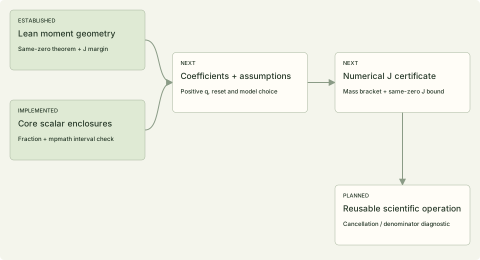
The proved moment geometry and implemented scalar enclosures feed the next coefficient and model-admissibility work. Their destination is a certificate for positive angular history at an exact mass zero.

Established Lean geometry and implemented scalar computations feed next coefficient and admissibility work, then a numerical J certificate and a planned scientific diagnostic.

Green: established or implemented. Light: next or planned. Arrows show research inputs.

04 / EQUATION TO ARTIFACT

The theorem is a milestone.
Useful scientific code is the destination.

The roadmap connects mathematical discovery to a callable computation, then to a measured scientific use. Each completed stage supplies an input for the next.

  1. ESTABLISHED

    1. Derive the mathematical mechanism

    Same-point M/J separation, a root-location-independent angular margin, normalized moments and a plateau lower bound.

    Theorems and proof records ↑
  2. IMPLEMENTED

    2. Make the core computation rigorous

    Exact-rational exponential enclosures, outward error bounds, deterministic outputs and rejection tests for modified records.

    Computed quantities ↑
  3. NEXT RESEARCH

    3. Certify an evaluable moment witness

    Enclose the repair coefficients, establish a positive numerical margin and connect admissible source inputs to the same-point moment result.

    Computational bridge plan ↗
  4. PLANNED TRANSFER

    4. Extract a reusable scientific primitive

    Turn cancellation, denominator margins or input-validity bounds into a function with explicit inputs, error assumptions and useful failure outputs.

    Candidate operations ↓
  5. PLANNED EVALUATION

    5. Test usefulness in a real workflow

    Compare against established numerical or research-software methods on the same workload. Measure error, diagnostic value, false alarms and cost.

    Application research plan ↗

Two routes to practical use

MATHEMATICAL COMPUTATION

Safer moment and ratio evaluation

A candidate diagnostic for scientific postprocessing: distinguish exact cancellation, unresolved near-cancellation and a usable denominator margin before returning a ratio. The first comparison is against stable summation, quadrature and conditioning checks.

RESEARCH WORKFLOWS

Make a reproduction failure actionable

A candidate tool for scientific-software teams: connect model, proof and execution changes to a concrete mismatch or regression. Evaluate it on real defect cases against existing Git, build and test diagnostics.

These are selected research directions. The next experiments determine which operations deliver measurable value in scientific or engineering workflows.

05 / READ THE WORK

Mathematics and implementation,
with distinct questions.

One object, two names: “angular moment” in P01’s title is the source H-weighted angular history J used on this page.

01 MATHEMATICS · P01 v0.5

A First-Repair Mass Zero Without Angular-Moment Cancellation

Yun Kwansub · 31 October 2026 · 11 pages · CC BY 4.0

For each fixed outgoing Profile, every sufficiently small positive parameter admits a point inside the first repair window where M = 0 and J > 0 at the same point. A weighted-tail comparison explains this separation and yields a positive lower bound independent of the qualifying zero’s location. The paper connects the source definitions, analytic argument and Lean propositions, including normalization and a cutoff-plateau bound.

Evidence: source-bound Lean propositions and fixed-checkpoint replay receipts.

Included in Software v0.5.0 · cdce801

Read paper PDF ↗
What changed in P01 v0.5?

The quantitative extension adds a zero-location-independent J margin, normalized second-bump moment identities and a conservative plateau lower bound: Theorems 3.3–3.4. The existing same-point existence result is retained.

Cite P01 v0.5 · BibTeX
Download .bib
@misc{yun_2026_23835054,
  author       = {Yun, Kwansub},
  title        = {A First-Repair Mass Zero Without Angular-Moment
                   Cancellation
                  },
  month        = oct,
  year         = 2026,
  publisher    = {Zenodo},
  version      = {0.5},
  doi          = {10.5281/zenodo.23835054},
  url          = {https://doi.org/10.5281/zenodo.23835054},
}

Official Zenodo export · version-specific DOI. Use the all-versions link to discover later editions.

02 RESEARCH SOFTWARE · P02 v0.6

From Source-Bound Proofs to Reproducible Research Artifacts: An NSRW Case Study

Yun Kwansub · 31 October 2026 · 10 pages · CC BY 4.0

This case study follows the moment investigation from proof inputs to retained execution artifacts. It explains fixed-checkpoint replay, fresh external modules and the resolution of actual invocation, elaboration and archive-preservation failures. Section 7.2 reports the 128/256/512-bit exact-rational core-scalar experiment and its error-bound method.

Evidence: recorded replay stages, documented incidents, software tests and retained scalar outputs.

One incident: a redundant tactic and ambiguous inequality types stopped a weighted-tail proof; the retry kept the theorem’s premises and conclusion.

Included in Software v0.5.0 · cdce801

Read paper PDF ↗
What changed in P02 v0.6?

Section 7.2 adds the exact-rational scalar experiment, stable positive-series expm1 evaluation and outward dyadic error bounds. The separate mpmath interval checker was added afterward; it is a subsequent software result, not an experiment reported in this manuscript.

Cite P02 v0.6 · BibTeX
Download .bib
@misc{yun_2026_23835112,
  author       = {Yun, Kwansub},
  title        = {From Source-Bound Proofs to Reproducible Research
                   Artifacts: An NSRW Case Study
                  },
  month        = oct,
  year         = 2026,
  publisher    = {Zenodo},
  version      = {0.6},
  doi          = {10.5281/zenodo.23835112},
  url          = {https://doi.org/10.5281/zenodo.23835112},
}

Official Zenodo export · version-specific DOI. Use the all-versions link to discover later editions.

Separate version tracks: v0.5.0 identifies the software release; P01 v0.5 and P02 v0.6 identify the manuscripts included in it. The PDFs match that release. The qualitative and quantitative proof executions have their own earlier checkpoints below.

P01 results → Lean declarations → replay checkpoints
Theorem numbers follow P01 v0.5. Each declaration link is fixed to its replay input.
P01 resultLean declaration / moduleExecution checkpoint
Theorem 3.1 · conditional mismatchangularMoment_pos_of_firstRepair_mass_zero
P2_ZPLUS_J_FirstRepairAngularMoment.lean
3a50b5f · 12 Oct
Theorem 3.2 · same-point existenceprofileMJ_firstRepair_zero_small_positive
P2_ZPLUS_J_SourceComposition.lean
3a50b5f · 12 Oct
Theorem 3.3 · quantitative marginangularMoment_ge_firstRepair_margin
P2_ZPLUS_J_QuantitativeMargin.lean
7f29ebf · 22 Oct
Theorem 3.4 · normalized plateau marginangularMoment_ge_plateau_margin
P2_ZPLUS_J_MarginNormalization.lean
7f29ebf · 22 Oct

Four quantitative and six normalization propositions support the extension. Open the replay receipts ↑

Using the workbench?

Cite the software release separately from the papers: v0.5.0 DOI · all software versions / latest · CITATION.cff.

Cite Software v0.5.0 · BibTeX
Download .bib
@software{yun_2026_23835493,
  author       = {Yun, Kwansub},
  title        = {Navier–Stokes Research Workbench},
  month        = oct,
  year         = 2026,
  publisher    = {Zenodo},
  version      = {v0.5.0},
  doi          = {10.5281/zenodo.23835493},
  url          = {https://doi.org/10.5281/zenodo.23835493},
}

Official Zenodo export · version-specific DOI. Use the all-versions link to discover later editions.

RESEARCH LIBRARY & WRITING

The work behind
the papers.

Read the working research

Browse the mathematical argument, computation methods, architecture and reproduction guides with a document sidebar and section index.

Open the research library ↗

Follow the ideas

From a scale-invariant candidate to an obstruction: what changed while reproducing a Navier–Stokes construction.

Explore the research writing ↗
06 / INSPECT · REPRODUCE · EXTEND

Follow the inputs.
Take the next step.

Inspect the argument

Start with the same-witness theorem, the weighted-tail comparison or the quantitative lower bound. Each result links to an exact Lean input and its execution receipt.

Proof records ↑

Run the computation

From the repository root, in a POSIX shell with Python ≥3.10:

PYTHONPATH=src python3 -m nsrw.math_kernel.p2_core_scalars produce --precision 128 --output core.json
PYTHONPATH=src python3 -m nsrw.math_kernel.p2_core_scalars verify --input core.json
Pinned Lean & numerical reproduction guide ↗

Contribute a precise review

Examine the same-witness quantifiers, source-coordinate correspondence, weighted-tail inequalities or exact-rational enclosure algorithm. A separately operated replay is also welcome.

Open a research review ↗
Exact scope of this research snapshot

The Lean results concern fixed Profiles of the pinned outgoing construction, with Profile-dependent positive thresholds and first-window witnesses. The numerical results enclose core scalars. Numerical coefficient positivity, an explicit source Profile, a root bracket and comparative application utility are subsequent tasks. Independent external reproduction remains open. Uniqueness, first-zero ordering, ratio poles and a general Navier–Stokes solution are outside the present results.